Excel WRAPROWS function

 

Excel WRAPROWS function

The WRAPROWS function converts a single row or column into multiple rows (a 2-demensional array) by specifying the number of values in each row.

Note: This function is only available in Excel for Microsoft 365 on the Insider channel.

Syntax

=WRAPROWS(vector, wrap_count, [pad_with])

Arguments

Vector (required): The array you want to warp into multiple rows.

Wrap_count (required): The maximum number of values for each row.

Pad_with (optional): A specified value to fill cells with no values. By default, #N/A error value will be displayed if there are insufficient elements to fill in.

Remarks

1) The #VALUE! error value occurs if “vector” is not a one-dimensional array (contains more than one column or row);

2) The #NUM! error value occurs if “wrap_count” is less than 1;

3) The #N/A! error value occurs if there are insufficient elements to fill the cells in columns.

4) If "wrap_count" is equal to or greater than the number of cells in the original array, the entire array will be returned in one row.

Return value

It returns an array wrapped by rows.

Example

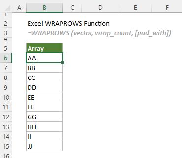
As shown in the screenshot below, to convert the one-dimensional array in the range B6:B15 into multiple rows, and each row contains at most 2 values, you can apply the WRAPROWS function to get it done.

Select a blank cell, such as D6 in this case, enter the following formula and press the Enter key to get the columns.

=WRAPROWS(A6:A15,2)

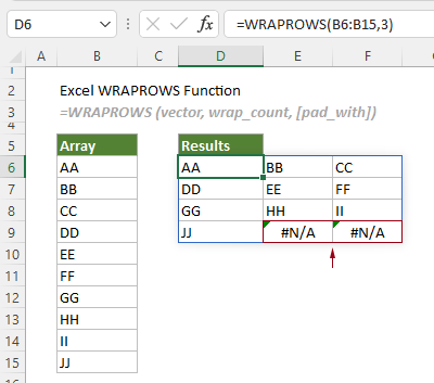
Notes: If you specify at most 3 values for each row, you will find that there are not enough values to fill the cells in the last row, so, #N/A is displayed.

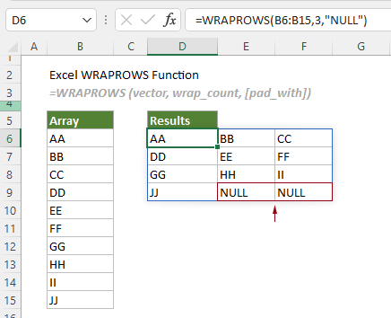
To replace the #N/A with a specified value, for example a word “NULL”, you need to specify the argument “pad_with” as “NULL”. See the formula below.

=WRAPROWS(A6:A15,2,"NULL")